
Ferrite cold demagnetization needs a curve review
Generic hard ferrite data shows a positive HcJ coefficient. Use the calculator to explore that trend; confirm your exact grade.
Evidence & scopeEstimate HcJ change with temperature, then review the grade data needed for a demagnetization decision.
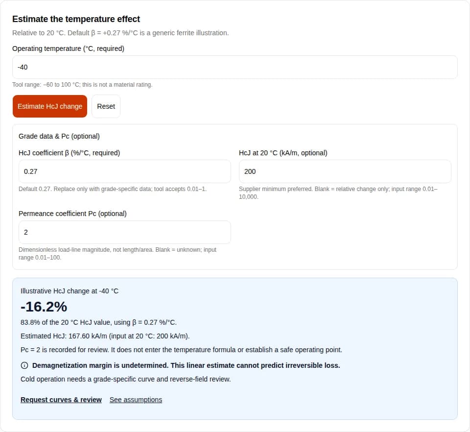
Relative to 20 °C. Default β = +0.27 %/°C is a generic ferrite illustration.
Generic hard ferrite data shows a positive HcJ coefficient. Use the calculator to explore that trend; confirm your exact grade.
Evidence & scopeA load-line value helps define the operating condition. It cannot establish a universal temperature or demagnetization limit.
Evidence & scopeMaterial selection needs temperature, reverse field and the curve shape. A single coercivity number is insufficient.
Evidence & scopeKeep the curve, units and reference temperature together. The Arnold material-selection presentation explains normal and intrinsic magnetic characteristics.
| Quantity | Meaning | Use here |
|---|---|---|
| HcJ / Hci | Reverse field magnitude at J = 0 on the intrinsic curve. | Optional baseline in kA/m at 20 °C. |
| HcB / Hc | Reverse field magnitude at B = 0 on the normal curve. | Do not substitute for HcJ. |
| Br | Remanent flux density at zero applied field. | Needed for the full operating-point review, not estimated here. |
| Pc | Magnitude of the normal load-line slope: |B/(μ₀H)| in SI; numerically |B/H| in gauss/oersted. | Dimensionless; circuit review context only. |
Unit conversion: 1 kA/m ≈ 12.566 Oe. If a report gives 2,500 Oe, enter approximately 198.94 kA/m. Pc is not magnet length divided by area; use a circuit calculation appropriate to the geometry. See Arnold’s Pc guidance.
ΔHcJ (%) = β × (T − 20)
HcJ(T) ≈ HcJ(20) × [1 + ΔHcJ (%) / 100]
β is entered in %/°C. The default +0.27 comes from Eclipse’s generic ferrite datasheet, page 2. It is an illustrative assumption for a barium ferrite enquiry, not a tested coefficient for your part. Replace it with documented grade data and its valid temperature interval.
| Item | Calculator treatment | Before design approval |
|---|---|---|
| Temperature | Accepted from −60 to 100 °C; reference 20 °C. | Confirm actual extremes and grade-specific coefficient validity. |
| HcJ and β | Optional baseline; constant coefficient assumption. | Obtain minimum properties and measured curves; interpolation may be needed. |
| Pc and reverse field | Pc is optional context; reverse field is not modeled. | Model assembly geometry, air gap, leakage and worst reverse field. |
| Flux loss / safety margin | Unknown; no safe/unsafe classification. | Define acceptance criteria and measure the assembled part. |
The tool’s numerical bounds prevent unsupported extrapolation; they do not certify any temperature interval. It covers an illustrative hard-ferrite trend, not powder, substituted research samples or a qualified bonded-magnet formulation. No probability of failure is calculated.
The local temperature trend does not justify extrapolation to the Curie transition. A rise in intrinsic coercivity also does not mean that remanence or useful assembly flux rises. Arnold’s temperature discussion separates these selection considerations.
These are calculated examples, not measured customer cases. For all three, assume HcJ(20) = 200 kA/m and β = +0.27 %/°C; the baseline is deliberately hypothetical.
| Scenario / assumption | Calculation | Estimate | Next action |
|---|---|---|---|
| Cold start: −40 °C | ΔT = −60; 0.27 × (−60) = −16.2%. | 167.60 kA/m; 83.8% of baseline. | Obtain the cold curve and check the maximum reverse field. |
| Reference check: 20 °C | ΔT = 0; change = 0.0%. | 200.00 kA/m; 100.0% of baseline. | Verify baseline units and minimum-versus-typical status. |
| Warm operation: 80 °C | ΔT = +60; 0.27 × 60 = +16.2%. | 232.40 kA/m; 116.2% of baseline. | Check Br, assembly temperature limits and coefficient validity. |
| Candidate | Available evidence | Decision requirement |
|---|---|---|
| Your barium ferrite grade | Baseline HcJ, β and cold curve: unknown until supplied. | Document composition, manufacturing route and minimum properties. |
| A strontium ferrite alternative | Family name alone does not quantify the improvement. | Compare the same geometry and operating condition using named grade curves. |
| NdFeB example: Arnold N42M | Datasheet lists HcJ ≥ 1,114 kA/m and coefficient −0.60 %/°C (measured over 20–100 °C). | Grade-specific example only; do not enter its negative coefficient in this ferrite tool. |
The NdFeB row is from Arnold N42M, revision 210607. It illustrates why changing material requires a new thermal review. No unsupported barium-versus-strontium numerical ranking is used.
The following are review actions proposed for this workflow; their benefit must be validated for the actual assembly.
| Risk | Potential consequence | Mitigation and tradeoff |
|---|---|---|
| Mistaking HcJ change for flux loss | An estimate is treated as an assembly acceptance result. | Specify post-cycle flux measurement and an allowable loss, including measurement repeatability. |
| Using an isolated-magnet Pc for an assembly | Steel, gap and opposing fields may change the operating condition. | Recalculate or simulate the assembled circuit; compare a geometry change with a documented higher-HcJ grade. |
| Switching grade without a cost comparison | A property gain may add tooling, volume or inspection expense. | Quote the same quantity and tolerances; include steel, assembly and testing in the comparison. |
| Applying sintered-ferrite assumptions to bonded parts | Binder and processing limits are omitted. | Request formulation-specific data or qualify a sintered alternative within the mechanical constraints. |
Published . Reviewed by FerriteCustom. Supplier literature supports the cited properties; calculations and review recommendations are identified separately. No independent measurements of your part are available. See our editorial and evidence policy.
It estimates the percentage change in intrinsic coercivity relative to 20 °C using a constant positive temperature coefficient. If you supply HcJ at 20 °C, it also returns an estimated kA/m value. It does not calculate demagnetization margin.
Yes, as an illustration only. Leave HcJ and Pc blank to keep unknowns explicit. The default coefficient is generic ferrite data, not a measurement of your barium ferrite part. Use the result to prepare a data request.
The tool refuses the calculation and offers a measured-curve request. These are limits chosen for this illustrative tool, not certified material limits. Even inside the range, confirm the coefficient over your actual temperature interval.
Pc describes the magnetic circuit load line; the percentage formula uses only temperature and the HcJ temperature coefficient. Pc is recorded as review context. Neither a high Pc nor this estimate proves that an assembly is safe.
No. HcB is the reverse field magnitude at which B reaches zero; HcJ is the reverse field magnitude at which intrinsic polarization J reaches zero. Enter the HcJ or Hci column from the supplier report, and keep its test temperature and units.
No. That is a change in the estimated coercive field, not an irreversible flux-loss prediction. Loss depends on the actual demagnetization curve, circuit and opposing field. Measure flux after a defined temperature cycle to establish loss.
Do not extrapolate this linear model to the Curie temperature. The local positive coefficient does not describe the full temperature dependence or guarantee retained magnetization near the magnetic transition.
No single value is suitable for acceptance. Composition, processing and measurement conditions matter. This page leaves your part’s baseline unknown until you enter a documented value, and does not relabel generic ferrite grades as barium-only specifications.
No. Compare named candidate grades using minimum HcJ, full curves at the required temperatures, Br, geometry and the same opposing-field condition. A material-family label is not an acceptance criterion.
It changes the circuit, but the improvement must be evaluated for the real air gap, contact, leakage and steel saturation. Recalculate the load line and test the revised assembly before accepting the change.
Request the material identity, minimum HcJ and Br with test temperatures, intrinsic and normal demagnetization curves, coefficient validity interval, dimensions, magnetization direction and lot traceability. Supply your worst reverse-field condition and allowable flux-loss criterion.
Request quotes at the same quantity, tolerances and inspection level. Compare magnet volume, tooling, added steel, assembly work and validation effort. This page contains no current price estimate; a cheaper part may need a more expensive assembly or test program.
Send the grade identity, dimensions and magnetization direction, minimum and maximum temperature, air gap or assembly sketch, and worst opposing field. Ask for minimum HcJ at the stated reference temperature and measured intrinsic/normal curves over your operating range.
If Pc is unknown, say so and send the geometry. Agree on allowed permanent flux loss, the thermal cycle, reverse-field exposure and measurement procedure before sample acceptance.
Inquiry Email
Copy the email, or open your default email app to start an inquiry.